
Servo systems are integral to a vast array of applications across the globe, from the intricate mechanisms in remote control devices and automotive steering to the sophisticated wing control systems in aircraft and the precise robotic arm manipulations in modern workshops. Available in diverse shapes, sizes, and power capabilities, servo operation is universally governed by the servo controller. This controller serves as the central hub, providing all necessary operational parameters to the servos. The industry is continuously evolving, with existing commercial entities developing advanced products to meet the ever-increasing demands of precision servo applications, and further innovations constantly emerging.
Components and Architectures of Servo Systems
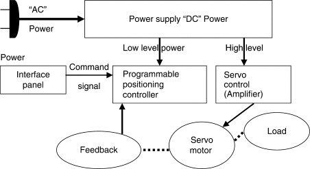
At its core, the term “servo” denotes a specific function or task within a system, as illustrated in Figure 4.31. The primary role of a servo system can be defined as follows: a command signal, initiated from a user interface panel, is received by the “positioning controller,” the brain of the servo system. This positioning controller is programmed to manage various tasks, storing information that dictates the activation of the motor or load—modifying its speed, position, or both.
 Concept of a servo system
Figure 4.31: Conceptual diagram illustrating the fundamental components and signal flow within a servo system.
The signal then progresses to the “servo control” or “amplifier” stage. Here, the low-power command signal is amplified to a level sufficient to drive the servomotor and the attached load. This amplification is crucial because higher voltage levels are required for faster motor speeds, and increased current levels are necessary to generate the torque needed to move heavier loads. The power required for this amplification is supplied to the servo control unit from a “power supply,” which converts standard AC power into the necessary DC voltage. This power supply also provides low-level voltage for the operation of integrated circuits within the system.
Upon receiving amplified power, the servomotor initiates movement, altering the speed and position of the load. Simultaneously, a feedback device, typically a tachometer, resolver, or encoder, monitors this movement. This device sends a “feedback” signal back to the positioning controller, informing it about the motor’s performance. The positioning controller analyzes this feedback signal to ascertain if the motor is executing the task correctly. If discrepancies are detected, the controller makes real-time adjustments to correct the motor’s operation.
In essence, a servo system is a combination of multiple devices working in concert to control a load. This control can be applied to various parameters such as position, direction, and speed. The regulation of speed or position is always relative to a reference, or command signal, and relies on accurate feedback from a detection device. By continuously comparing the feedback and command signals and implementing corrections, the system ensures precise control. Therefore, to Define Servo System precisely: it is an integrated system composed of several components designed to control or regulate the speed and position of a load with high accuracy and responsiveness.
Logic Circuits in Servo Controllers
The resurgence of Radio Controlled (R/C) servos, particularly among robotics enthusiasts, has highlighted the importance of efficient servo controllers. Operating these versatile servos requires the generation of stable Pulse Width Modulated (PWM) control signals, which can be complex to manage, especially in multichannel applications. A streamlined solution involves employing a dedicated serial servo controller board. This board manages the intricacies of multichannel PWM signal generation and is controlled via simple commands transmitted through a standard serial UART interface. Advanced designs, such as a 32-parallel-channel system, integrate the processing power of an FPGA (Field-Programmable Gate Array) with the intelligent capabilities of an MCU (Microcontroller Unit) to achieve superior performance specifications.
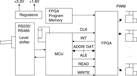
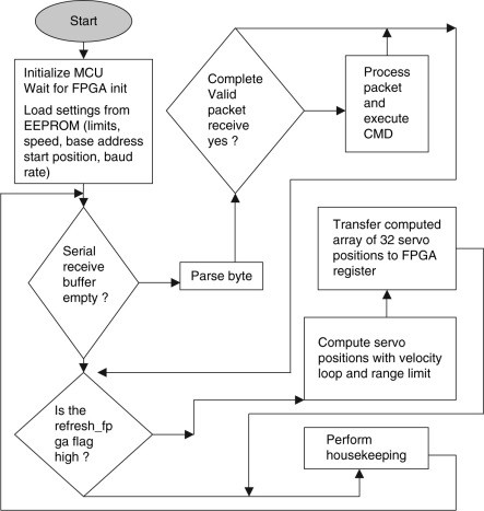
Figure 4.32 provides a block diagram illustrating the logic circuits of a typical serial servo controller. Within an FPGA, a 32-channel parallel array of 16-bit accuracy, 12-bit resolution PWM generation units is implemented. An MCU is central to the system’s operation. Its external memory bus is effectively utilized to interface with a memory-mapped array of 64 PWM registers (32 channels × 16 bits) within the FPGA. The MCU performs multiple critical functions, including initializing FPGA registers with user-defined servo startup positions stored in internal EEPROM. Upon receiving an external interrupt at each PWM cycle, the MCU refreshes all current servo position values in the FPGA’s memory-mapped PWM registers through a direct memory-to-memory transfer, as depicted in Figures 4.33 and 4.34.
 Overall serial servo controller circuit block diagram
Figure 4.32: Block diagram illustrating the overall circuit architecture of a serial servo controller.
 Internal architecture of FPGA for serial servo controller
Figure 4.33: Detailed internal architecture of the FPGA component within the serial servo controller circuit.
 MCU firmware flowchart for serial servo controller
Figure 4.34: Flowchart outlining the MCU firmware operation for the serial servo controller circuit.
Open Loop vs. Closed Loop Servo Systems
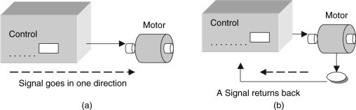
In a servo system, motion initiation is managed by the controller, which sends commands to the motor to start or adjust speed, position, or both. This command is then amplified and applied to the motor, resulting in motion. Servo systems can be broadly categorized into open loop and closed loop configurations, as shown in Figure 4.35.
 Open loop and close loop drive
Figure 4.35: Diagram comparing (a) Open loop drive system and (b) Closed loop drive system configurations in servo control.
Open Loop Systems: Systems operating under the assumption that motion occurs as commanded are termed “open loop.” In an open loop drive, the control signal flows unidirectionally from the controller to the motor. There is no feedback mechanism to confirm if the intended motion has actually taken place.
Closed Loop Systems: Conversely, systems that incorporate feedback are known as “closed loop.” These systems operate bidirectionally: a command signal is sent to move the motor, and a feedback signal is returned to the controller, providing confirmation of the action taken. This feedback loop allows the system to monitor and adjust performance in real-time.
Limitations of Open Loop Systems: Open loop systems are less suitable for applications with variable loads, and stepper motors in such systems can lose steps, leading to inaccuracies. They are also generally less energy-efficient and prone to resonance issues that must be carefully avoided.
Advantages of Closed Loop Systems: Closed loop systems are preferred for applications requiring precise control over complex motion profiles, including velocity and/or position control, high resolution and accuracy, and operations at both very slow and very high velocities. They are also essential for applications demanding high torque in compact designs.
While the added complexity and cost of feedback components in closed loop systems might be perceived as drawbacks, the enhanced control, accuracy, and adaptability they offer often outweigh these considerations, especially in demanding applications. The choice between open and closed loop servo systems often depends on the specific requirements of the application and the user’s priorities.
Control Mechanism of Servo Systems
Servo control is fundamentally the regulation of a motor’s velocity and position based on feedback signals. The most basic servo loop is the velocity loop, which generates a torque command to minimize the discrepancy between the commanded velocity and the actual velocity feedback. For most servo systems, position control is also crucial. This is commonly achieved by adding a position loop in cascade or series with the velocity loop. In simpler configurations, a single PID (Proportional-Integral-Derivative) position loop can manage both position and velocity control without a separate velocity loop.
Servo loops require “tuning” for optimal performance in each specific application. Tuning involves adjusting servo gains. Higher gains can enhance performance but also increase the system’s susceptibility to instability. Low-pass filters are often integrated in series with the velocity loop to mitigate high-frequency stability issues. These filters must be tuned in conjunction with the servo loops. To address particularly challenging applications, some drive manufacturers provide advanced control algorithms that can overcome the limitations of standard servo loops imposed by system mechanics or stringent performance requirements.
Motor control, in the context of servo systems, refers to the process of generating actual torque in response to torque commands from the servo control loops. For brush motors, this is primarily achieved by controlling the current in the motor winding, as torque is directly proportional to current. Most industrial servo controllers utilize current loops, which are structurally similar to velocity loops but operate at much higher frequencies. A current loop compares a current command (typically from the velocity loop output) with a current feedback signal and generates a voltage command. To increase torque, the current loop increases the voltage applied to the motor until the desired current level is reached. Current loop tuning is typically performed by manufacturers for specific motors, relieving users of this complex task.
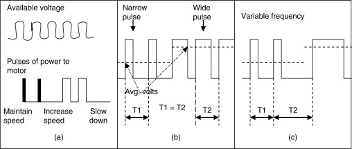
One type of semiconductor device used in servo control is the Silicon Controlled Rectifier (SCR), which can be connected to the AC line voltage, as shown in Figure 4.36(a). SCRs are typically used in high-power applications where precise speed control is not critical, such as constant speed devices for fans, blowers, and conveyor belts. Power delivery from an SCR to the motor is in discrete pulses. Maintaining low speeds requires a continuous stream of narrow pulses, while increasing speed necessitates larger pulses of instant power. Reducing speed involves cutting off power and allowing the motor to coast down. This on-off control results in a somewhat jerky operation, analogous to towing a car with a chain – control is lost when slack occurs in the chain during deceleration. While adequate for many applications, this method lacks smoothness.
 Servo control types: SCR, PWM, and PFM
Figure 4.36: Illustration of servo control types: (a) SCR control, (b) Pulse Width Modulation (PWM), and (c) Pulse Frequency Modulation (PFM).
For smoother speed control, electronic networks, such as a “lag” network, can be implemented. These networks slow down the control response, preventing sudden power surges. The filtering action of a lag network makes the motor respond sluggishly to rapid changes in load or speed commands. This sluggishness is acceptable in applications with steady loads or high inertia but is undesirable in high-performance systems requiring rapid response to speed command changes.
Transistors offer another method for regulating power to motors. Several techniques exist for transistor-based control, including linear mode, Pulse Width Modulation (PWM), and Pulse Frequency Modulation (PFM).
Linear Mode: In linear mode, transistors are continuously active, modulating power like a faucet to supply the exact amount needed. A partially activated transistor delivers a fraction of the power, while a fully activated transistor delivers maximum power. This continuous power delivery, unlike SCR control, results in smoother speed stability and control.
Pulse Width Modulation (PWM): PWM regulates power by applying pulses of variable width, as shown in Figure 4.36(b). Narrow pulses result in lower average voltage and slower motor speeds, while wider pulses increase average voltage and speed. PWM offers the advantage of reduced power loss in the transistor, as it operates primarily in fully “ON” or “OFF” states, minimizing heat dissipation and allowing for more compact designs.
Pulse Frequency Modulation (PFM): PFM regulates power by varying the frequency of power pulses, as depicted in Figure 4.36(c). Fewer pulses per unit time result in lower average voltage and slower speeds, while more frequent pulses increase average voltage and speed.
Distributed Servo Control Systems
The configuration of servo motion systems, integrating both hardware and software, is highly application-dependent, leading to a vast array of possible setups. Motion controllers are available that operate across multiple platforms and buses, offering analog outputs for conventional amplifiers and direct PWM outputs for up to 32 motors simultaneously. Amplifiers may still require potentiometers for adjusting position, velocity, and current control in digital drives. This modularity allows for near-limitless combinations to achieve tailored solutions for specific applications.
Ongoing advancements in hardware are driving the development of faster and more precise motion control products. New microprocessors and Digital Signal Processors (DSPs) facilitate enhanced features, functionality, and performance at reduced costs. These enhancements, such as increasing the number of axes on a motion controller or integrating position controls into drives, are directly attributable to progress in electronics. As servo and motion control performance improves, system-level requirements become more demanding. Machines employing servo actions now routinely incorporate more sophisticated software and complex functions on host computers. Competitive differentiation among servo and motion system providers increasingly hinges on the quality of their operating systems.
Traditional servo systems often comprise a high-power front-end computer communicating with a high-power, DSP-based multiaxis motion controller card, which interfaces with multiple drives or amplifiers, often equipped with their own high-end processors. Communication levels between the host computer and motion controller can be categorized into: simple point-to-point moves with non-critical trajectories; moves requiring coordination and trajectory blending linked to machine operation; and complex moves with process-critical trajectories.
A growing trend is the integration of motion control functionality into compact modules for mounting near motors, creating distributed systems. Centralizing communication links from these controller/amplifiers to the computer significantly reduces system wiring, lowering costs and improving reliability. By increasing power stages, a single unit can independently drive multiple motors, limited only by the DSP’s processing capacity. If size reductions are sufficient, distributed servo controller/amplifiers can be placed outside control panels, potentially further reducing system costs.
Implementing a distributed servo controller and amplifier requires meeting several key system requirements: sufficient processing power for multiaxis control, high-speed communication with the host computer, compact size for distributed deployment, and cost-effectiveness.
Levels of Motion Complexity in Distributed Control: Distributed servo controllers and amplifiers must cater to varying levels of motion complexity. For point-to-point moves with non-critical trajectories, two types of distributed systems are relevant: one for repetitive moves triggered by external events, and another for variable destinations based on user or machine-generated events. A typical application is a “pick and place” robot, used for tasks ranging from silicon wafer handling to parts assembly and packaging.
Distributed servo controller and amplifier requirements for such applications involve trajectory determination based on current location and either user-defined or preprogrammed destinations. Typically, users only need to set acceleration, velocity, jerk parameters (for S-curves), and a series of final points.
Minimal host-controller communication is needed, primarily for simple commands and feedback. Key features include a resident motion program for path planning, I/O functionality support, RS-232 terminal interface, operation without a resident editor/compiler, and stand-alone motion control. Complete motion control applications can be programmed into the distributed control module for stand-alone operation in three-axis applications, commonly used in machines requiring simple, repetitive sequences controlled via an RS-232 terminal.
Communication in stand-alone mode is typically straightforward and not time-critical. Simple RS-232 communication is adequate for systems with few motors, while multidrop RS-485 or RS-1394 is suitable for applications with numerous axes and motor networks.
For “blended moves with important trajectories,” more extensive host computer communication is necessary due to increased information and critical feedback speed and detail. Computerized Numerical Control (CNC) machining, requiring accurate and repeatable path cuts, exemplifies this. Trajectory generation and following must be smooth for quality cuts. Distributed servo control modules must support full coordination of multiple axes. Host communication is critical, as latency between command issue and motor response can cause motion inconsistencies.
Coordination between multiple motors can be achieved in several ways. A single distributed servo controller and amplifier module with multiple amplifiers can manage coordination internally. For applications requiring coordination across motors connected to different controllers, a high-bandwidth network is necessary.
Trajectory Planning for Complex Motions: Applications involving complex moves with critical trajectories, such as inverse kinematics in robotics, often incorporate proprietary trajectory planning. Trajectory generation is performed on a computer platform, and the information is transferred to the motion controller. Significant engineering effort is invested in top-level robot software that pre-calculates trajectories and transmits this data to the controller, potentially underutilizing conventional motion controller capabilities.
For distributed servo controllers and amplifiers in such scenarios, the interface involves sending a series of set points over the network for the controller to follow, interpolating for higher resolution. Servo drives are configured for torque, speed, or position control. Solutions like smart cards in the PC with DeviceNet and FireWire options are added to support synchronized motion profile streaming (Profile Streaming Mode) for users requiring arbitrary trajectory specification.
System integration in motion control continues to advance, pushing demands for faster controllers with high-speed multiaxis capabilities in multitasking applications across all major value-adding components.
Important Servo Control Devices
Key components in servo control systems include motors and feedback devices.
(1) Types of Motors: Electric motor design is based on the principle of conductors placed in a magnetic field. A winding, comprising many wire turns, amplifies the interaction. The force generated by a winding depends on the current and magnetic field strength. Increased current yields greater force (torque). Motor action arises from the interaction of two magnetic fields: the rotor and stator fields attract each other, forming the basis for both AC and DC motor designs.
(a) AC Motors: AC motors typically operate at relatively constant speeds determined by the applied voltage frequency and the number of magnetic poles. Two primary types exist: induction and synchronous motors.
(i) Induction Motor: An induction motor can be understood as a type of transformer. Applying voltage to the primary winding (stator) induces current in the secondary winding (rotor). A magnetic field in the stator induces another in the rotor, and their interaction causes motion. The stator’s rotating magnetic field dictates rotor speed, with the rotor “slipping” behind when loaded. Thus, induction motors always rotate slightly slower than the stator field.
Construction typically includes a laminated stator with copper wire windings and a “squirrel cage” rotor made of steel laminations with conductive material (copper or aluminum) in peripheral slots, short-circuited by conductive end pieces, often with integral cooling fan blades.
Standard induction motors operate at constant speeds from fixed line frequencies. However, demand for adjustable speed drives has led to controls using microprocessor technology (vector or phase angle control, variable voltage, variable frequency) to manipulate magnetic flux magnitude and control motor speed. With appropriate feedback sensors, induction motors become viable for certain positioning applications. However, speed and torque control becomes complex as torque is no longer a simple function of current, affecting slip frequency, and speed depends on both stator field and slip frequencies.
(ii) Synchronous Motor: Synchronous motors are similar to induction motors but with modified rotor construction, enabling them to rotate synchronously with the stator field. Two subtypes exist: self-excited and directly excited (permanent magnet).
Self-excited (reluctance synchronous) motors have rotors with peripheral notches or teeth (salient poles) corresponding to stator poles. These salient poles create easy magnetic flux paths, allowing the rotor to “lock in” and synchronize with the rotating field.
Directly excited (hysteresis synchronous or AC permanent magnet synchronous) motors use a rotor with a permanent magnet alloy cylinder. The permanent magnet poles act as salient teeth, preventing slip.
Both types exhibit a “coupling” angle—rotor lag behind the stator field—which increases with load. Exceeding motor capability causes the rotor to lose synchronism (“pull-out”). Synchronous motors typically operate in open loop and provide constant speed for a given load within coupling angle limits (pull-out torque). They are not self-starting, requiring start windings (split-phase, capacitor start) or controls for gradual frequency and voltage ramp-up.
Synchronous motors can be used in speed control systems with added feedback. Vector control is applicable, but generally, rotors are larger than servomotors, potentially limiting response in incrementing applications. Other disadvantages include potential failure to accelerate high inertial loads into synchronism, leading to low-frequency, irregular, noisy operation, and larger size and higher cost compared to nonsynchronous motors for the same horsepower.
(b) DC Motors: DC motors are easily speed-varied, making them suitable for speed control, servo control, and positioning applications. Stator fields are generated by field windings or permanent magnets (stationary field). Rotor fields are created by current through a commutator into the rotor assembly. The rotor field rotates to align with the stator field, but the commutator switches the rotor field at appropriate times, preventing alignment and causing continuous rotation. Rotational speed depends on rotor field strength (motor voltage).
DC motor types include shunt wound, series wound, compound wound, stepper motor, and permanent magnet DC (PMDC) motors.
(i) Shunt Wound Motors: Rotor and stator (field windings) are connected in parallel. Field windings can be powered by the same or separate supply as the rotor. Separate excitation allows speed adjustment by varying rotor voltage while keeping field winding voltage constant.
Parallel connection provides a relatively flat speed-torque curve and good speed regulation across wide load ranges. However, starting torque is lower than other DC types due to demagnetization effects.
(ii) Series Wound Motors: Rotor and stator fields are connected in series, resulting in strong fields and very high starting torque. Field windings carry full rotor current. Used in high starting torque applications like cranes and hoists. Avoid in no-load conditions due to “run away” tendency.
(iii) Compound Wound Motors: Use both series and shunt stator fields. Speed-torque curves vary with series/shunt field ratio.
Small compound motors typically have strong shunt and weak series fields for starting assistance, exhibiting high starting torque and relatively flat speed-torque characteristics. Reversing applications require switching polarity of both windings, necessitating complex circuits.
(iv) Stepper Motors: Electromechanical actuators converting digital inputs to analog motion via controller electronics. Types include solenoid activated, variable reluctance, permanent magnet, and synchronous inductor.
All stepper motors index in fixed angular increments when programmed. Normal operation is discrete angular motion, not continuous. Well-suited for pulse train controller signals; one pulse increments one angle of motion. Mostly used in open loop, which can cause oscillations. Closed loop systems use complex circuits or feedback to mitigate oscillations.
Stepper motors are limited to about one horsepower and 2000 rpm, restricting their use in many applications.
(v) PMDC Motors: Permanent Magnet DC (PMDC) motors are prevalent in demanding incrementing (start-stop) applications. With feedback, they are effective in closed loop servo systems.
Stator fields are generated by permanent magnets, requiring no field generation power. Magnets provide constant field flux at all speeds, resulting in linear speed-torque curves.
PMDC motors offer high starting/acceleration torque, linear and predictable performance, smaller frame size and lighter weight, and rapid positioning capabilities.
(2) Types of Feedback Devices: Servos use feedback signals for stabilization, speed, and position information, provided by devices like analog tachometers, digital tachometers (optical encoders), and resolvers.
(a) Analog Tachometers: Resemble miniature motors but are not power-delivering devices. Shaft rotation generates voltage at terminals (motor in reverse). Voltage magnitude is proportional to speed; polarity indicates rotation direction.
Analog (DC) tachometers provide directional and rotational information, used for speed indication and velocity feedback. Simplest method for velocity feedback.
Example: Lead screw assembly at 3600 rpm. Tachometer output gradient 2.5 V/Krpm. Expected voltage: 3.6 Krpm × 2.5 V/Krpm = 9V. Servo drive maintains this voltage for desired speed.
Tachometer characteristics include voltage constant, ripple, and linearity.
- Voltage Constant: (Voltage gradient, sensitivity) Output voltage at 1000 rpm (V/Krpm or V/rad/s).
- Ripple: AC signal superimposed on DC output due to manufacturing tolerances. Defined as peak-to-peak, RMS, or peak to average percentage of DC level.
- Linearity: Deviation of actual voltage-speed curve from ideal straight line, due to manufacturing tolerances. Maximum difference between actual and theoretical curves.
(b) Digital Tachometers: (Optical encoders, encoders) Mechanical-to-electrical conversion devices. Shaft rotation produces output signal proportional to rotation angle/distance. Output signals can be square waves, sinusoidal waves, or absolute position data. Types: absolute and incremental.
(i) Absolute Encoder: Provides unique address for each shaft position (360°). Uses contact (brush) or noncontact (photoelectric) sensing.
Contact scheme uses brushes to contact conductive paths on coded disk. Noncontact scheme uses photoelectric detection of coded disk position.
Resolution/accuracy increases with track count on coded disk. Built-in “memory” – position information retained during power failure, no need to return to “home” position after power restoration.
(ii) Incremental Encoder: Provides pulses or sinusoidal output as shaft rotates (360°). Distance data obtained by counting pulses.
Disk with opaque lines. Light source through transparent segments onto photosensor, outputting sinusoidal waveform, converted to square pulse train electronically.
Important parameters:
- Line Count: Pulses per revolution. Determined by required positional accuracy.
- Output Signal: Sine or square wave.
- Number of Channels: One or two. Two-channel provides signal relationship for motion direction (clockwise/counterclockwise). Zero index pulse for “home” position determination.
Example application: Counter loaded with desired position. Encoder pulses increase with motor acceleration until constant run speed. Pulses relate directly to motor speed. Counter counts pulses, motor slows down at predetermined location to prevent overshoot. Motor stops when counter is within 1-2 pulses of desired position. Load positioned.
(3) Resolvers: Resemble small motors. Signal winding rotor revolves in fixed stator. Transformer type device: exciting one winding excites the other. Rotor movement changes stator output, proportional to rotor angle.
Basic resolver: Single rotor winding, two stator windings (90° apart). Reference signal to rotor (primary), coupled to stator (secondary) via transformer action. Secondary output sine wave proportional to angle (other winding cosine wave). One electrical cycle per 360° mechanical rotation. Signals fed to controller.
Resolver to Digital (R to D) converter in controller analyzes signal, outputting rotor angle and speed.
Resolver types: Single speed (one sine wave per 360° rotor rotation), multi-speed (e.g., four-speed – four sine waves per 360°).
Synchronizer: Three stator windings (120° apart).
Resolver subtypes:
- Resolver Transmitter (CX, RCS): Single-phase input, two-phase outputs. Rotor winding excited, stator windings provide position information.
- Resolver Control Transformer (CT, RCT, RT): Two-phase inputs, single-phase output. Stator windings excited, rotor winding provides position information.
- Differential Resolver (RD, RC): Two-phase inputs, two-phase outputs. Rotor windings excited, stator windings provide position information.