
Building upon our previous exploration, “Deep Learning Deployment Artifact—Triton Inference Server Getting Started Guide“, this article continues our journey into Triton Inference Server, a critical tool for efficient deep learning model deployment.
For deployment engineers, or anyone aiming for streamlined model deployment, mastering Triton Inference Server is becoming an essential skill. Once your models are optimized, Triton takes center stage to handle the complexities of serving them.
It’s important to note that when we mention Triton here, we are referring to Triton Inference Server, not OpenAI’s Triton. They are distinct entities.
This is the second article in our Triton series. We’ll delve into fundamental concepts like inference, inference engines, inference frameworks, and service frameworks. We will also discuss practical aspects of deployment and how Triton’s features significantly accelerate your inference pipelines, enhancing both resource utilization and throughput.
This article will focus on two key Triton features:
- Dynamic Batching
- Concurrent Model Execution
In real-world applications, these features are instrumental in achieving higher resource utilization, reducing latency, and increasing throughput for your models.
Understanding Inference: The Core Concept
Let’s clarify what inference entails. Deep learning workflows generally consist of two phases: training and inference. Training is concerned with updating model weights and backpropagation of gradients. Inference, on the other hand, involves using a trained model to make predictions. It’s the process of feeding input data through the model’s operations to obtain an output result.
model = centernet_res50()
dummy_input = torch.randn(1, 3, 1024, 1024)
output = model(dummy_input)
output_box = nms(output)
This Python code snippet demonstrates a simple inference process in PyTorch. Typically, post-processing steps like Non-Maximum Suppression (NMS) are also involved. This entire pipeline, including preprocessing, model execution, and post-processing, is crucial for evaluating the model’s accuracy. We assess if the model meets our requirements by comparing its predictions (e.g., bounding boxes) with ground truth labels.
Once validation is complete and the model’s performance (e.g., mAP for object detection) is satisfactory, the next step is to utilize the trained model. Common use cases include:
- Offline Tasks: Processing a batch of queries over a period to accomplish a specific task. For example, using an object detection model trained on the COCO dataset to filter images containing people.
- Online Services: Deploying models online for users to access and utilize.
- Local Execution: Real-time applications like autonomous driving, where models are invoked as needed.
All these scenarios necessitate model inference, similar to the code example shown earlier.
Real-World Inference Considerations
Real-world inference is more complex than the simplified example. Several critical factors come into play:
- Model Accuracy: The model’s predictions must be accurate and meet the required performance metrics.
- Inference Speed: Faster inference (lower latency) is always desirable.
- Hardware Utilization: Maximize the utilization of hardware resources (GPU and CPU) during inference. Avoid idle resources.
- Stability: The inference process should be stable, preventing crashes, core dumps, or memory overflows.
- Determinism: Except for specific cases like chatbots, inference should ideally be deterministic. Given the same input, the model should produce the same output, eliminating randomness.
Let’s elaborate on these points:
Model Accuracy and Performance Metrics
Deployment often involves converting models from training frameworks like PyTorch to optimized formats like ONNX or TensorRT. It’s crucial to ensure that this conversion process preserves the model’s accuracy and minimizes any performance degradation compared to the original PyTorch implementation.
Inference Speed and Latency
Inference speed, or latency, is paramount. For instance, a PyTorch model might take 30ms to process a 1024×1024 image on an NVIDIA 3080 GPU. Converting the same model to TensorRT could reduce this latency to just 7ms, a significant 4x speedup. This 7ms represents the inference latency.
Deterministic Results
For most models (convolutional, fully connected, self-attention based), consistent output for the same input is expected. If you encounter inconsistent results, first check your input data and post-processing steps. Hardware issues could also be a rare cause.
Hardware Utilization and Stability
Hardware utilization and stability are influenced by both the inference framework and the service framework (like Triton). The inference framework (e.g., TensorRT, PyTorch LibTorch) dictates the model execution speed and resource utilization. TensorRT, for example, often achieves higher GPU utilization than directly running PyTorch models. Triton Inference Server plays a vital role in managing and optimizing hardware utilization and ensuring stable inference.
To clarify, an inference framework typically encompasses an inference engine. The engine handles the low-level execution, while the framework manages API interactions, input/output processing, and overall workflow.
Consider the example of deploying a NanoDet object detection model using LibTorch:
std::vector<boxinfo> NanoDet::detect(cv::Mat image, float score_threshold, float nms_threshold) {
    // Input: Preprocess the image to get model input
    auto input = preprocess(image);
    // Net: Model, forward pass to get outputs
    auto outputs = this->Net.forward({input}).toTensor();
    // Post-processing: Decode outputs to get bounding boxes
    torch::Tensor cls_preds = outputs.index({ "...",torch::indexing::Slice(0,this->num_class_) });
    torch::Tensor box_preds = outputs.index({ "...",torch::indexing::Slice(this->num_class_ , torch::indexing::None) });
    std::vector<:vector>> results;
    results.resize(this->num_class_);
    this->decode_infer(cls_preds, box_preds, score_threshold, results);
    std::vector<boxinfo> dets;
    for (int i = 0; i < this->num_class_; ++i) {
        nms(results[i], nms_threshold);
        for (auto box : results[i]) {
            dets.push_back(box);
        }
    }
    return dets;
}
This C++ code snippet illustrates a complete inference pipeline: preprocessing, model forward pass (Net.forward), and post-processing. It takes an image as input and returns detected bounding boxes.
While writing basic inference code like this is feasible, achieving high performance and throughput in real-world scenarios requires more sophisticated design. Simply using LibTorch might not fully utilize hardware resources. We can measure inference speed with a simple timer:
#include <chrono>
auto startTime = std::chrono::high_resolution_clock::now();
nanodet.detect(image, 0.5, 0.4);
auto endTime = std::chrono::high_resolution_clock::now();
float totalTime = std::chrono::duration<float, std::milli>(endTime - startTime).count();
Benchmarking with loops often reveals that LibTorch might not saturate the GPU, reaching only 60-70% utilization. This indicates potential GPU waste. Converting the model to TensorRT can improve speed and utilization. Furthermore, concurrent requests using multi-threading can further boost throughput.
This is where service frameworks like Triton Inference Server come into play. They encapsulate inference frameworks (like LibTorch) and provide features for high-performance, high-throughput deployments.
Service frameworks, sometimes referred to as serving frameworks or inference servers, abstract away the complexities of managing inference workloads.
Both the initial PyTorch example and the LibTorch example can be deployed using Triton to achieve optimized performance. Refer to the official Triton documentation for detailed tutorials.
Concurrent Model Execution in Triton Inference Server
Triton’s architecture is designed to execute multiple models and/or multiple instances of the same model concurrently on a single system. An “instance” in this context corresponds to a thread, representing a single execution of the NanoDet::detect function in our example. Real-world deployments often involve multiple models (e.g., object detection and classification models).
The diagram below illustrates concurrent execution of two models: model0 (detection) and model1 (classification).
 Triton Mult-Model Execution Diagram
If Triton is idle and two inference requests arrive simultaneously, one for each model, Triton immediately schedules both on the GPU. The GPU’s hardware scheduler then handles the parallel processing of these computations.
CPU-based models are handled similarly by Triton, with the operating system managing thread scheduling on the CPU.
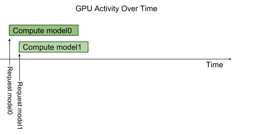
By default, if multiple requests arrive for the same model (e.g., two requests for model1), Triton serializes their execution, processing them one after another on the GPU, as shown below.
 Triton Mult-Model Serial ExecutionDiagram
Triton offers a model configuration option called instance-group to control the level of parallelism for each model. Each enabled parallel execution is termed an instance. By default, Triton provides one instance per model per available GPU. The instance_group field in the model configuration allows you to adjust the number of execution instances for a model. The following diagram shows model execution when model1 is configured to allow three instances. The first three requests for model1 are executed in parallel. The fourth request must wait for one of the first three to complete.
 Triton Mult-Model Parallel ExecutionDiagram
This example is analogous to running four threads: one for model0 requests and three for model1 requests. Essentially, four models can be executed concurrently due to the four parallel threads, maximizing GPU and CPU utilization.
It’s important to remember that concurrent execution in Triton doesn’t inherently speed up individual model inference. It primarily aims to maximize resource utilization and increase throughput by keeping the hardware busy. The underlying model inference speed remains unchanged.
Dynamic Batching for Increased Throughput
Batching is a common technique to improve GPU utilization. NVIDIA demos often use ResNet-34 classification models with large batch sizes like 64x3x224x224.
High batch sizes are used because they effectively saturate the GPU, showcasing NVIDIA hardware’s capabilities. GPUs are inherently designed for massive parallel computations, and larger batches simplify CUDA algorithm design, enabling efficient utilization of Streaming Multiprocessors (SMs).
Larger batches also enhance the utilization of Tensor Cores, further boosting performance on NVIDIA GPUs that have them.
Therefore, maximizing batch size in model inference is crucial for improving utilization and throughput. Triton Inference Server supports dynamic batching, which intelligently combines incoming inference requests into dynamically formed batches to enhance processing efficiency.
Your models must, of course, support batching. For example, a model might be designed to accept input tensors with a shape like (-1, 3, 256, 256), where -1 indicates a variable batch dimension.
Let’s illustrate dynamic batching with an example (see diagram below).
Assume five inference requests (A, B, C, D, E) with batch sizes of 4, 2, 2, 6, and 2, respectively. Each batch takes X milliseconds to process by the model (assuming processing time is X ms regardless of batch size, as long as it’s within the model’s maximum batch size of 8). The requests arrive in this order: A and C at time T=0, B at T=X/3, and D and E at T=2X/3.
Diagram illustrating the benefits of dynamic batching compared to no batching.
Without dynamic batching, requests are processed sequentially, taking 5X milliseconds in total. This is inefficient as the model has the capacity to process larger batches.
Dynamic batching optimizes request scheduling and GPU memory utilization, reducing the total processing time to 3X milliseconds in this example. It also reduces latency as more queries are processed in less time.
Triton allows setting a delay parameter for grouped batching, called “Delay”. This instructs Triton to wait for a certain duration after receiving a request to accumulate a larger batch before sending it to the model. For example, the following configuration sets a maximum delay of 100 milliseconds:
dynamic_batching {
  max_queue_delay_microseconds: 100
}
With a delay, Triton can group requests A, B, and C together, and D and E together, forming larger batches and further improving resource utilization (see “dynamic batching / delay=X/2” in the diagram).
Note that this is an idealized example. In practice, not all execution steps are perfectly parallelizable, and large batches might sometimes lead to longer execution times due to factors like memory bandwidth limitations.
Dynamic batching enhances both response speed and processing capacity when serving models. This feature is primarily designed for stateless models (like object detection models, where each inference is independent). For stateful models, Triton offers sequence batching, which we will discuss in a future article.
Combining Dynamic Batching with Concurrent Model Execution (multiple instances) further amplifies performance. For example, with two instances of a model:
Diagram showing dynamic batching with two model instances.
Without dynamic batching, requests are distributed across available model instances. Users can also set priorities to influence instance scheduling.
With dynamic batching and multiple instances, query B can be processed by the second instance as it arrives. By setting a delay for instance 1, it can be filled to its maximum batch size and launched at time T=X/2. Simultaneously, queries D and E, accumulating to fill the maximum batch size, allow the second model instance to start inference immediately without waiting.
Triton Inference Server provides flexible batching strategies, improving resource utilization, reducing latency, and increasing throughput. Deploying your models with Triton ensures they are operating at their full potential.
For practical examples, refer to the official Triton documentation.
Conclusion
A Triton backend is the implementation that executes a model. A backend can be a wrapper around deep-learning frameworks like PyTorch, TensorFlow, TensorRT, or ONNX Runtime. It can also be custom C/C++ logic for operations like image pre-processing.
This article provided an overview of Triton’s operations and optimizations for inference pipelines, focusing on dynamic batching and concurrent execution. The next article will delve into the backend details of Triton, exploring how it encapsulates inference code and manages multi-threading for efficient execution.